Chapter 2: Relational Model¶

1. The Introduction of relational model¶

a brief conclusion¶

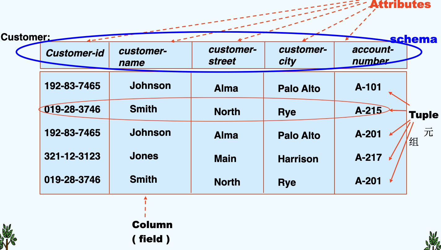
an example of Relation¶

2. Basic Structure¶

definition¶

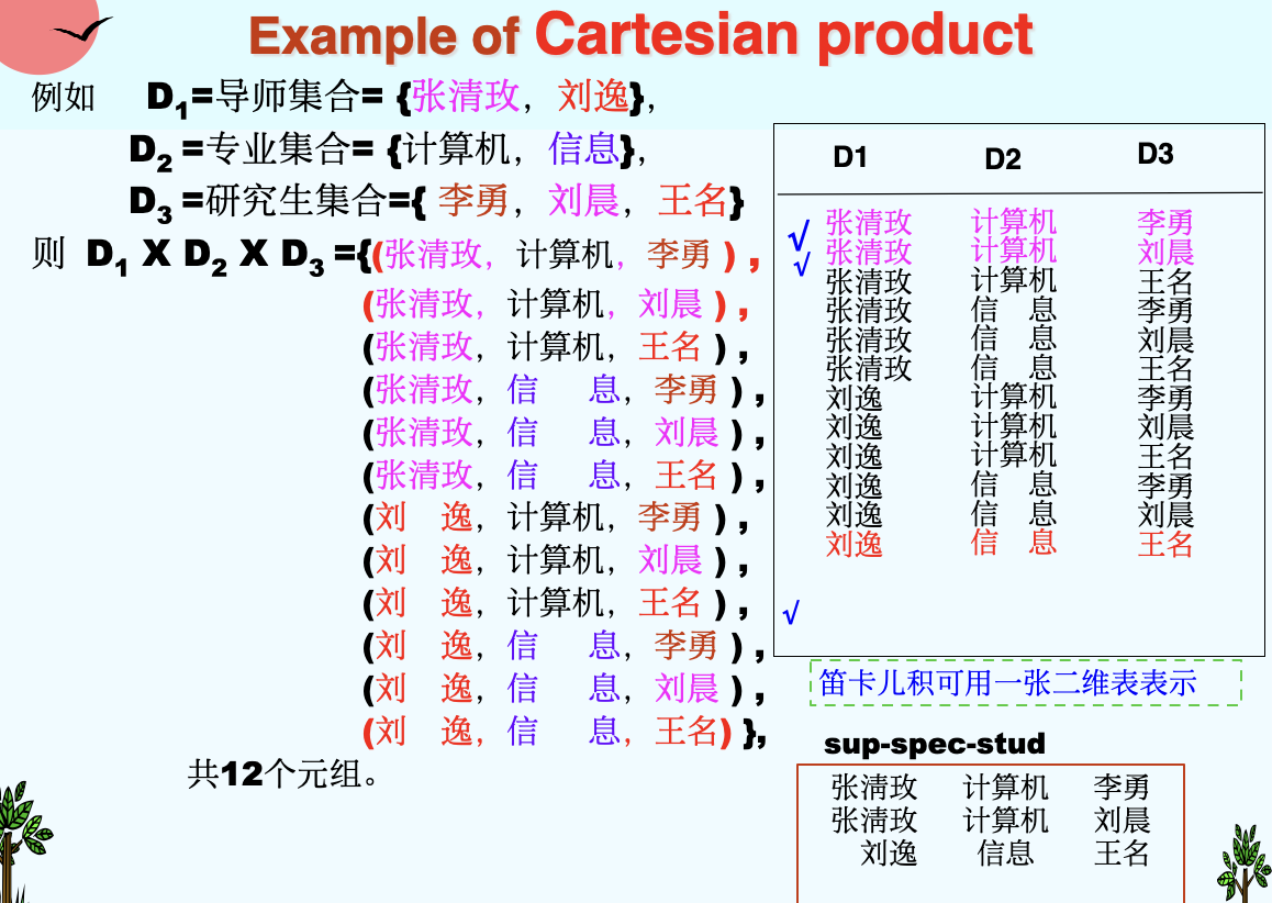
1. Formally, given sets \(D_1, D_2, ..., D_n\), \(D_i = a_{ij}|_{j=1...k}\)
2. a relation r is a subset of \(D_1 \times D_2 \times ... \times D_n\)

3. a Cartesian product of a list of domain \(D_i\)

4. Thus a relation is a set of n-tuples(\(a_{ij}, a_{2j}, ..., a_{nj}\))

An Example of Cartesian product¶

(1)Attribute Types¶

1. Each attribute of a relation has a name.
2. The set of allowed values for each attribute is called the domain (域) of the attribute.
3. Attribute values are (normally) required to be atomic, that is, indivisible. (1st NF, 第一范式)
4. E.g. multivalued attribute values are not atomic
5. E.g. composite attribute values are not atomic
6. The special value null is a member of every domain.
7. The null value causes complications in the definition of many operations.
   • we shall ignore the effect of null values for the moment and consider their effect later.

(2)Concepts about relation¶

1. A Relation is concerned with two concepts : relation schema and relation instance.
2. The relation schema describe the structure of the relation.
3. The relation instance corresponds to the snapshot of the data in the relation at a given instant in time.
4. C.f.: Database schema and database instance.

(2-a) Relation Schema¶

1. \(A_1, A_2, ..., A_n\) are attributes
2. Formally expressed:
   • \(R = (A_1, A_2, ..., A_n)\) is a relation schema
   • E.g. Instructor-schema = (ID, name, dept_name, salary)
3. \(r(R)\) is a relation on the relation schema R

(2-b) Relation Instance¶

1. The current values (relation instance) of a relation are specified by a table.
2. An element t of r is a tuple, represented by a row in a table.

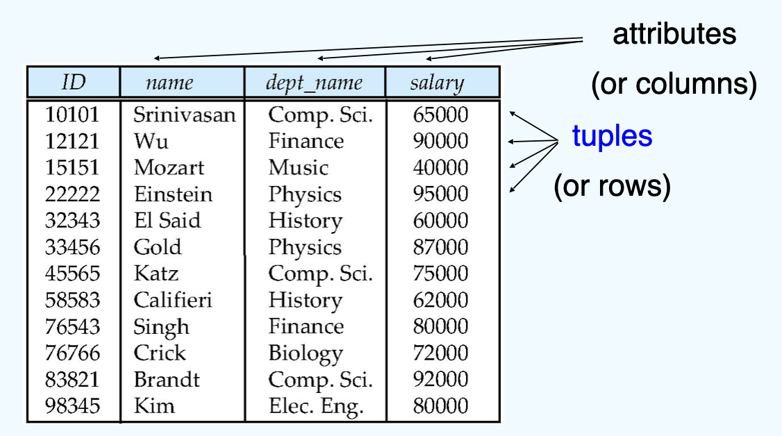
• Let a tuple variable t stands for a tuple. Then t[name] denotes the value of t on the name attribute.

(3) Relations are Unordered¶

1. Order of tuples is irrelevant (tuples may be stored in an arbitrary order), and tuples in a relation are no duplicate(完全一样的).
2. E.g. department(dep_name, building, budget) relation with unordered tuples.

(4) Keys(码、键)¶

1. Let \(K \subseteq R\)
2. K is a superkey(超码) of R if values for K are sufficient to identify a unique tuple of each possible relation r(R)
   • Example: {instructor-ID, instructor-name} and {instructor-ID} are both superkeys of instructor.
3. K is a candidate key(候选码) if K is minimal superkey.Example: {instructor-ID} is a candidate key for instructor, since it is a superkey, and no subset of it is a superkey.
4. K is a primary key(主码), if k is a candidate key and been defined by user explicitly. Primary key is usually marked by underline.

(5) Foreign key(外键，外码)¶

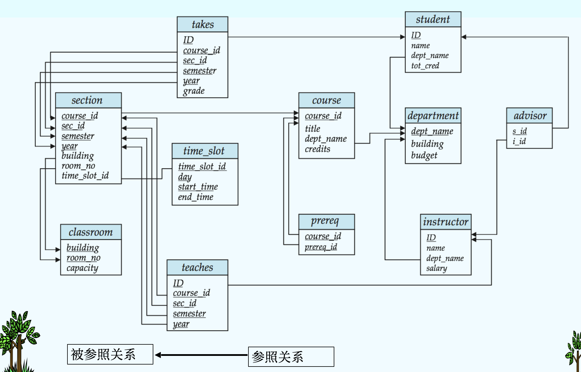
• Assume there exists relation r and s: r(A, B, C), s(B, D), we can say that attribute B in relation r is foreign key referencing s, and r is a referencing relation(参照关系) , and s is a referenced relation(被参照关系).

(6) Schema of the University Database¶

• classroom(building,room_number,capacity)
• department(dept_name,building,budget)
• course(course_id,title,dept_name,credits)
• instructor(ID,name,dept_name,salary)
• section(course_id,sec_id,semester,year,building,room_number,time_slot_id)
• teaches(ID,course_id,sec_id,semester,year)
• student(ID,name,dept_name,tot_cred)
• takes(ID,course_id,sec_id,semester,year,grade)
• advisor(s_ID,i_ID)
• time_slot(time_slot_id,day,start_time,end_time)
• prereq(course_id,prereq_id)

(7)Query Languages¶

1. Language in which user requests information from the database.
2. “Pure” languages:
   • Relational Algebra - the basis of SQL
   • Tuple Relational Calculus (元组关系演算)
   • Domain Relational Calculus - (域关系演算) QBE
3. Pure languages form underlying basis of query languages that people use, e.g. SQL.

3. Relational Algebra¶

1. Procedural language (in some extent).
2. Six basic operators
   • Select 选择
   • Project 投影
   • Union 并
   • set difference 差（集合差）
   • Cartesian product 笛卡儿积
   • Rename 改名（重命名）
3. The operators take one or two relations as inputs and give a new relation as a result.
4. Additional operations
   • Set intersection 交
   • Natural join 自然连接
   • Division 除
   • Assignment 赋值

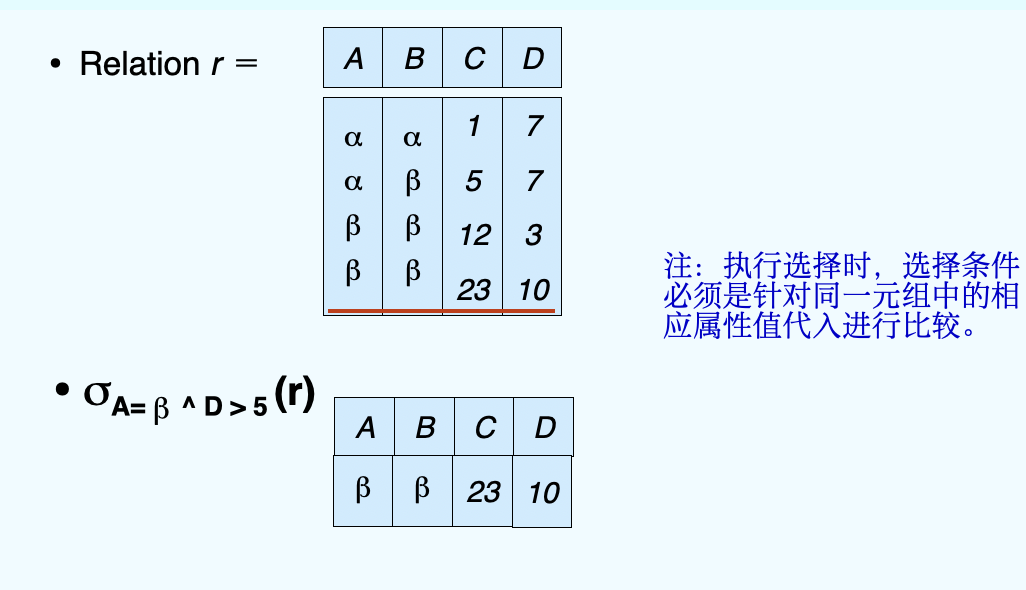
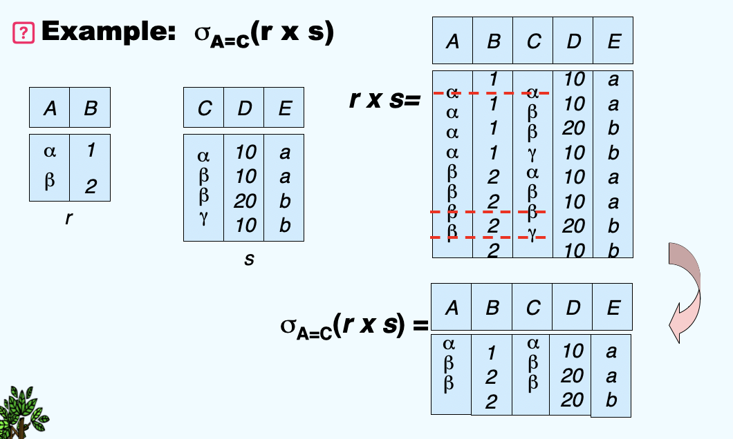
(1)Select Operation¶

1. Notation: \(\sigma_p(r)\), \(\sigma\) is pronounced as sigma
2. p is called the selection predicate
3. Defined as: \(\sigma_p(r) = {t|t\in r and p(t)}\)
   • Where p is a formula in propositional calculus consisting of terms connected by: ∧ (and), ∨ (or), ¬ (not)
   • Each term is one of: op or , where op is one of: =, ≠ , >, ≥ , < , ≤
4. Example of selection: \(\sigma_{dept\_name='Finance'}(department)\)

Let's show an example below:

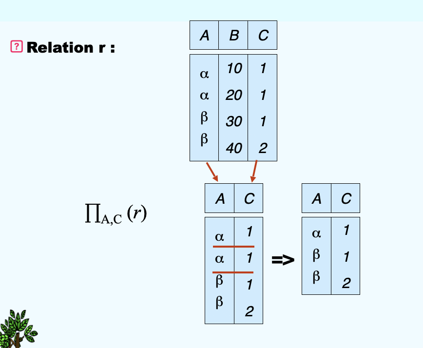
(2)Project Operation¶

1. Notation:\(\prod_{A1, A2, ... Ak}(r)\), \(\prod\)is pronounced as pi, where \(A_1, … A_k\) are attribute names and r is a relation name
2. The result is defined as the relation of k columns obtained by erasing the columns that are not listed
3. Duplicate rows removed from result, since relations are sets.
4. E.g. To eliminate the building attribute of department, we can use: \(\prod_{building}(department)\)

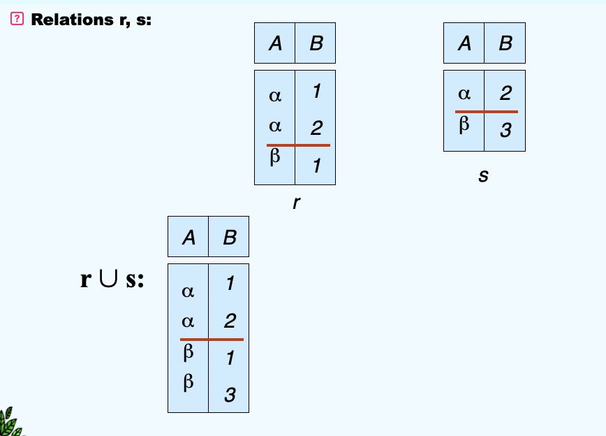
(3)Union Operation¶

1. Notation: \(r\cup s\)
2. Defined as: \(r\cup s = {t|t\in r \; or \; t\in s}\)
3. For \(r\cup s\) to be valid:
   • r, s must have the same arity (same number of same attributes)
   • The attribute domains must be compatible (e.g., 2nd column of r deals with the same type of values as does the 2nd column of s)

(4)Set Difference Operation¶

1. Notation: \(r - s\)
2. Defined as: \(r - s = \{t | t\in r \ \ {and} \ \ r \notin s\}\)
3. Set differences must be taken between compatible relations.
   • r and s must have the same arity
   • attribute domains of r and s must be compatible

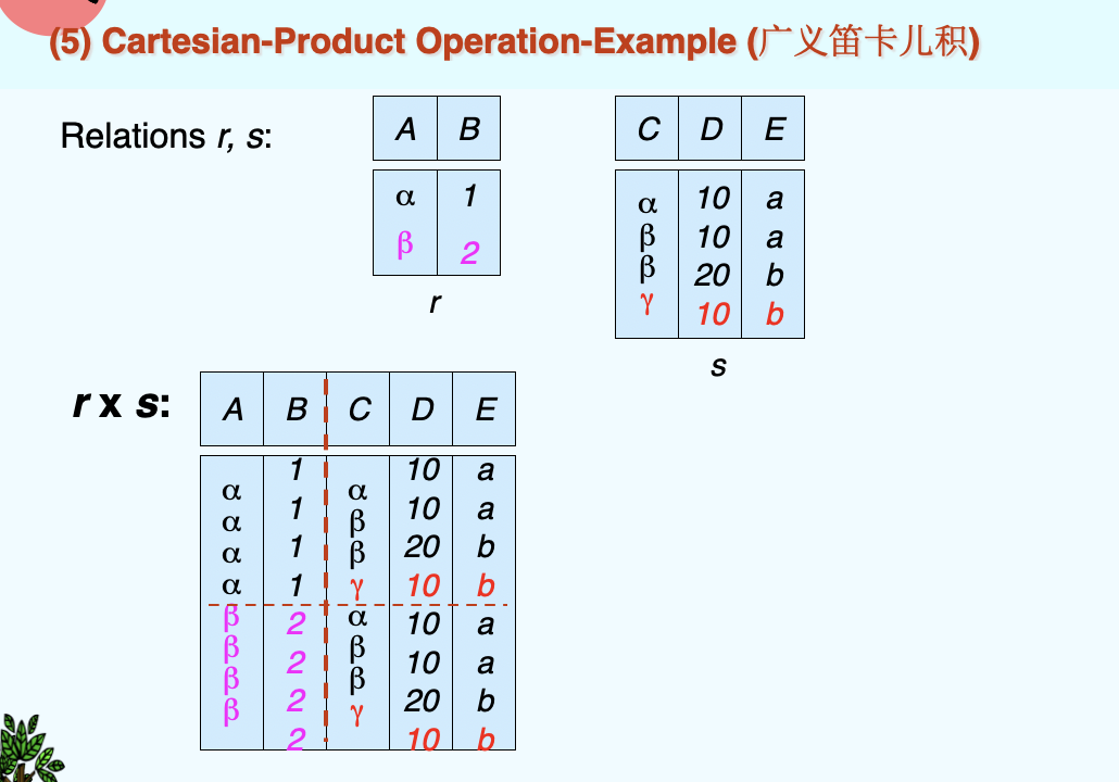
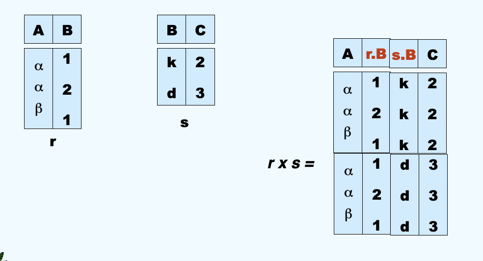
(5)Cartesian Product Operation(广义笛卡尔积)¶

1. Notation: \(r \times s\)
2. Defined as: \(r \times s = \{ \{t \ q \}\ t \in r \ \ {and} \ \ q \in s\}\)
3. Assume that attributes of r(R) and s(S) are disjoint. (That is, \(R \cap S = \emptyset\))
4. If attributes of r(R) and s(S) are not disjoint, then renaming for attributes must be used.

(6)Composition of Operation¶

• Can build expressions using multiple operations

(7)Rename Operation¶

1. Allows us to name, and therefore to refer to, results of relational-algebra expressions.
2. Allow us to refer to a relation by more than one name.

3. Then we can have two examples below:

   • \(\rho_X(E)\), \(\rho\) is pronounced as rho returns the expression E under the name X
   • If a relational-algebra expression E has arity n, then \(\rho_{X(A1, A2, ..., An)}(E)\) returns the result of expression E under the name X, and with the attributes renamed to \(A1, A2, ..., An\)

4. We have an example below:

Basic information:

branch (branch-name, branch-city, assets)

customer (customer-name, customer-street, customer-city)

account (account-number, branch-name, balance)

loan (loan-number, branch-name, amount)

depositor (customer-name, account-number)

borrower (customer-name, loan-number)

Queries:

Find the names of all customers who have a loan at the Perryridge branch.

Query1: \(\prod_{customer-name}(\sigma_{branch-name = "Perryridge"(\sigma_{borrower.loan-number = loan.loan-number}(borrow\times loan))})\)

Query2: \(\prod_{customer-name}(\sigma_{borrower.loan-number=loan.loan-number}(borrower\times (\sigma_{branch-name="Perryridge"}(loan))))\)

Above are two kinds of queries, which one is better?

The second is better: when it comes to \(\times\), the fewer tuples a relation has, the better it participates in the operation.

1. 找最大/最小时，先作笛卡尔积，然后用总集减去其补集

below are some additional operations

(8)Set-Intersection Operation¶

1. Notation: \(r \cap s\)
2. Defined as: \(r \cap s = \{t|t\in r \ \ and \ \ t\in s\}\)
3. Assume:
   • r, s have the same arity
   • attributes of r and s are compatible
4. Note: \(r \cap s = r-(r-s)\)

(9)Natural-Join Operation¶

1. Notation: \(r ⋈ s\)

2. Example:

   • R = (A,==B==,C,==D==); S = (E,==B==,==D==)
   • Result schema of natural-join or r and s = (A, ==B==, C, ==D==, E);
   • \(r ⋈ s = \prod_{r.A, r.B, r.C, r.D, s.E}(\sigma_{r.B = s.B \land r.D = s.D}(r \times s))\)

3. 它和笛卡尔积的辨析：笛卡尔积对于不同relation中的同名attributes选择了换名都保留，但是这个是只取相同部分

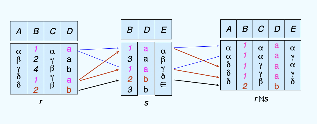
1. Theta join: \(r\ \mathop{\bowtie}\limits_{\theta}\ s = \sigma_{\theta}(r\times s)\)

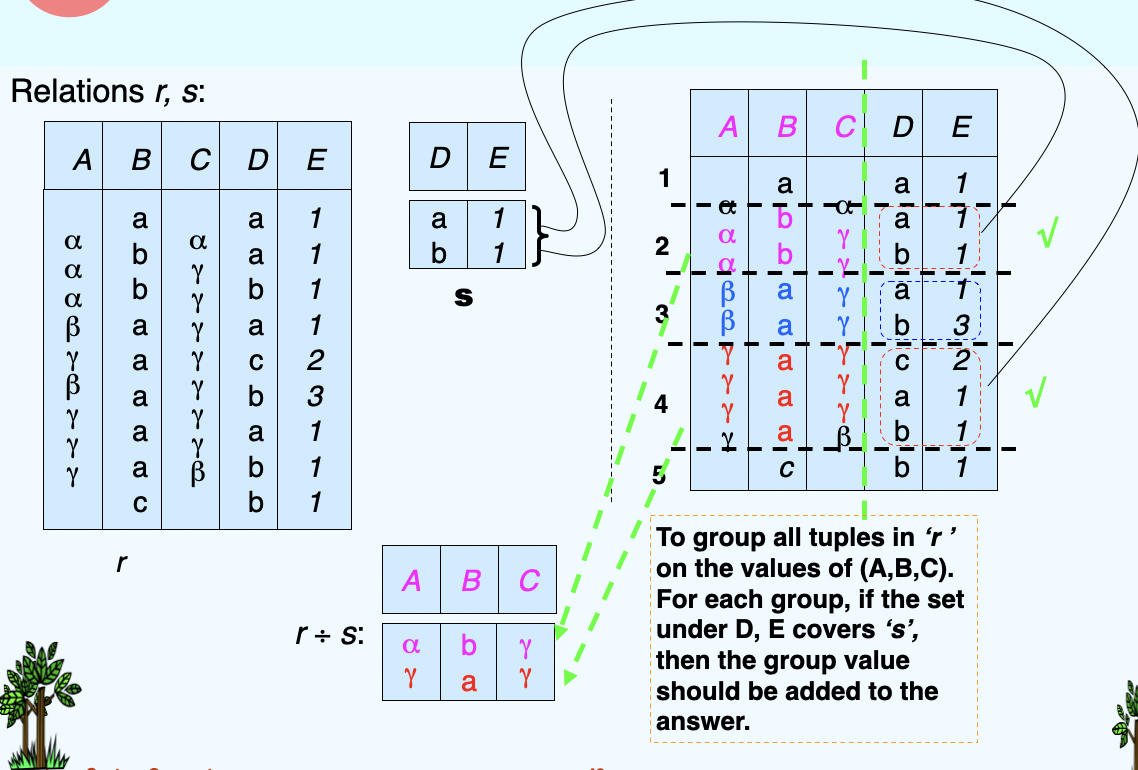
(10)Division Operation¶

• Let r and s be relations on schemas R and S respectively where
  • R = (\(A_1\), ..., \(A_m\), \(B_1\), ..., \(B_n\))
  • S = (\(B_1\), ..., \(B_n\))
• The result of \(r \div s\) is a relation on schema \(R-S = (A_1, ..., A_m)\)
  • \(r \div s = \{t \ | \ t\in \prod_{R-S}(r) \ \land \ \forall u \in s (tu\in r)\}\)

(11)Assignment Operation¶

1. The assignment operation (\(\leftarrow\)) provides a convenient way to express complex queries
   • Write query as a sequential program consisting of a series of assignments, which is followed by an expression whose value is displayed as a result of the query.
   • Assignment must always be made to a temporary relation variable
2. Example: Write \(r\div s\) as:
   • temp1 \(\leftarrow\) \(\prod_{R-S}(r)\)
   • temp2 \(\leftarrow\) \(\prod_{R-S}((temp1\times s)-\prod_{R-S,S}(r))\)

4. Extended Relational-Algebra-Operations¶

(1)Generalized Projection¶

1. Extends the projection operation by allowing arithmetic functions to be used in the projection list: \(\prod_{F1, F2, ..., Fn}(E)\)
2. E is any relational-algebra expression
3. Each of \(F_1, F_2, ..., F_n\) are arithmetic expressions involving constants and attributes in the schema of E.

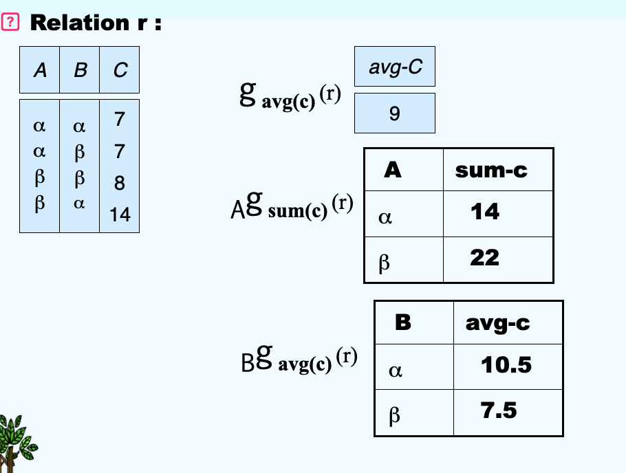
(2)Aggregate Functions and Operations¶

1. Aggregation function takes a collection of values and returns a single value as a result.
2. Aggregation operation in relational algebra: \(G_1, G_2, ..., G_n \ g \ F1(A1), F2(A2), ..., Fn(An)(E)\)
   • \(E\) is any relational-algebra expression
   • \(G_1, G_2, ..., G_n\) is a list of attributes on which to group(can be empty)
   • Each \(F_i\) is an aggregate function
   • Each \(A_i\) is an attribute name

An example:

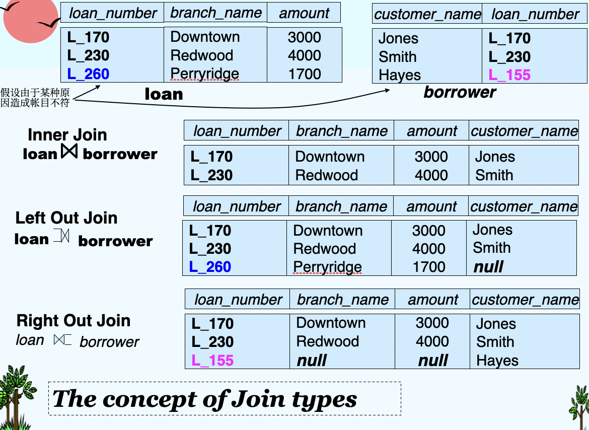
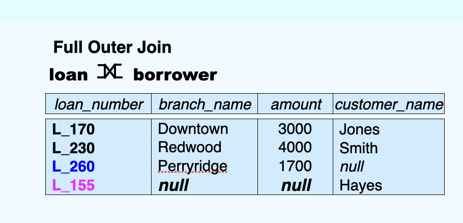
(3)Outer Join¶

1. An extension of the join operation that avoids loss of information.
2. Computes the join and then adds tuples form one relation that does not match tuples in the other relation to the result of the join.
3. Uses null values:
   • null signifies that the value is unknown or does not exist
   • All comparisons involving null are (roughly speaking) false by definition.
     • Will study precise meaning of comparisons with nulls later

Below I will show several kinds of outer join types: An example:

(4)Null Values¶

1. It is possible for tuples to have a null value, denoted by null, for some of their attributes
2. null signifies an unknown value or that a value does NOT exist.
3. The result of any arithmetic expression involving null is null.
4. Aggregate functions simply ignore null values
   • Is an arbitrary decision. Could have returned null as result instead.
   • We follow the semantics of SQL in its handling of null values
5. For duplicate elimination and grouping, null is treated like any other value, and two nulls are assumed to be the same
   • Alternative: assume each null is different from each other
   • Both are arbitrary decisions, so we simply follow SQL

(5)Modification of the Database¶

1. The content of the database may be modified using the following operations:
   • Deletion: \(r \leftarrow r - E\)
   • Insersion: \(r \leftarrow r \cup E\)
   • Updating: \(r \leftarrow \prod_{F1, F2, ..., Fi}(r)\)